Previous articles have discussed the use of statistics in tolerance analysis: how statistical summation works, how to account for the influence of different distributions, and how to combine worst-case with statistical contributions. The resulting picture is that the outcome of the analysis can be quite dependent on the assumptions you make. As a product designer, however, you don’t always know in advance how accurately the parts will be produced. Therefore, your analysis is only as good as the assumptions you make in it. However, if you work with the process capability index Cpk, your analysis will be more accurate.
Better Products and Analysis with Process Capability Index Cpk
Six Sigma is an excellent system for controlling dimensional deviations of parts. An important part of it is the determination of the so-called process capability index Cpk. Parts (products) manufactured with a Cpk requirement (almost) always have dimensional deviations with a Normal (Gauss) distribution. The process capability index Cpk, popularly called ‘the Cpk’, is a measure of the distance of this Normal distribution from the (tolerance) specification. The Cpk can be used for all kinds of parameters in your production process and ultimately leads to a (more) controlled process, among many other things. Lower failure rate and also more efficient.
The Calculation of the Cpk
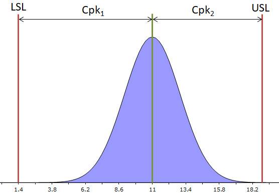
Before we start using the Cpk in tolerance analysis, a brief explanation of how the Cpk is calculated is needed. As mentioned before, the Cpk says something about the distance of the Normal distribution from the (tolerance) specification. The figure below illustrates this. In it, LSL is the lower specification limit and USL is the upper specification limit. In practice, these are your tolerance limits. Notice that Cpk is the relative distance. In formula form, the Cpk is: Cpk1 = (μ – LSL)/3σ and Cpk2 = (USL – μ)/3σ. Where μ = mean value (center of the Normal distribution) and σ is the standard deviation. The smaller of the two is ‘the Cpk’.
Using Cpk, Do You Have all the Information Now?
So if you know the Cpk of the parts in your tolerance analysis, you can easily use that? The answer is yes and no. Yes, because you can assume that the mean value of all your dimensional deviations is exactly zero. No, because you are making another assumption. If you know the Cpk, you still don’t know what the mean deviation μ is. And you need that in your tolerance analysis.
Now you can do two things:
- Specify in advance what the maximum deviation from the mean μ can be.
- Make an assumption about the maximum deviation from the mean μ.
Obviously, 1) is preferable. This is because then you know exactly what the possible deviations are. If 1) is not possible, then you will have to make an assumption. That’s not a bad thing, many (manufacturing) companies do it. A common method is the Six Sigma method mentioned above.
Six Sigma Method, a Brief Overview
The Six Sigma methodology was developed by Motorola in 1986 based on observations in their manufacturing operations. They saw that even in well controlled processes, the mean values μ showed some drift. And the maximum drift was quantified by Motorola as +/-1.5σ. It may sound strange that the drift of the mean is a factor of the standard deviation σ. But if you think about it, it actually makes sense. It would be strange if you had a very accurate process, a small σ, with a large drift. And vice versa. The name of the method comes from the specification limits: +/-6σ. The figure below illustrates this. A Six Sigma compliant process has a Cpk of 1.5 (=(6σ-1.5σ)/3σ).
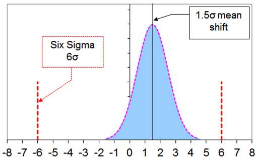
Interestingly, further, the maximum expected failure rate is 3.4 ppm (3.4 x 10⁻⁶). Note that due to drift, only one-sided exceedances of the 6σ limit play a role. Also, the distance from the mean to the 6σ limit is only 4.5σ. If you just want to check this in MS Excel, you can use this formula:
=NORM.DIST(-4.5,0,1,TRUE) or =1-NORM.DIST(4.5,0,1,TRUE).
Using Cpk in Your Tolerance Stack-Up Analysis
So, if the (allowable) mean deviation μ is not known, you can use the value μ=1.5σ as many other companies do. Let’s put this into the formula for the Cpk, and let’s also say that the LSL and the USL are equal to your (symmetrical!) tolerance specification ‘Tol’. Then, after reworking, you get: σ = Tol / (1.5 + 3Cpk). If you want to use the factor k (μ=kσ) instead of 1.5, then you get: σ = Tol / (k + 3Cpk). Since you almost always calculate with 3σ, you still have to multiply this answer by 3.
You now have two columns in your tolerance table for each degree of freedom. One with the 3σ value and one with the expected maximum drift μ. You can easily add up the 3σ values statistically, but how do you add up the individual drift values?
Stack-up Drift in Your Tolerance Table. And put it in a Template!
Drift is often not a phenomenon that can be easily averaged. Thus, statistical summation is not realistic. On the other hand, worst-case addition is again very pessimistic. It is unlikely that drift will always be maximally unfavorable for all parts in your tolerance chain. So something in between? Yes, something in between seems best. I prefer the assumption that the drift μ is randomly distributed for each part in your tolerance chain. Not too optimistic by statistically adding up, nor too pessimistic by considering the drift as worst-case.
Randomly distributed is the same as uniformly distributed. And uniformly distributed values can be statistically added with a correction factor. For uniformly distributed values, the correction factor is exactly √3. There is no need to figure all this out yourself. All this thinking and calculating is standard in the TolStackUp template, available here on the site.