A previous article discussed statistical tolerance stack-up analysis. It is usually more profitable to perform a statistical tolerance stack-up analysis instead of a worst-case analysis. A worst-case analysis often leads to low tolerance specifications and therefore high(er) costs.
Gaussian Distribution or Not?
A statistical tolerance stack-up analysis often assumes a Gaussian distribution of tolerances. But is that a realistic assumption? This depends on the actual variation and the tolerances used. The question that needs to be answered is: is the process for achieving the dimensional tolerance specification balanced (under control, perfectly matched to the required accuracy) or not? Basically, there are three possibilities.
- Yes, it is a well balanced process step. The Gaussian distribution is an reasonable assumption.
- No, the process step is not balanced and the tolerance specification is much wider (or narrower) than the capability of the actual process. For example: the tolerance specification is +/-0.5 mm, while it is a simple milling process with an actual variation of +/-0.1 mm.
- No, the process step is not balanced and the required accuracy is quite difficult to achieve. The Gaussian distribution is too optimistic.
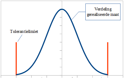
Normal Process with Gaussian Distribution
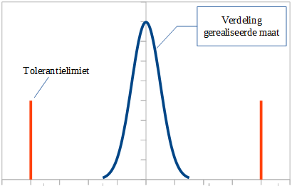
Process with Narrow Gaussian Distribution
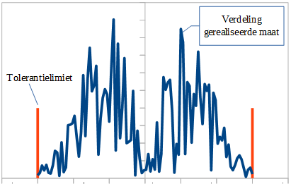
Distribution of an Uncontrolled Process
What to Choose, Statistical or Something Else?
In case 1, it is also important to realize that the mean of the dimension may be off-center with respect to the desired dimension. Also, the actual distribution is unlikely to be 100% perfect Gaussian. All of these deviations can be corrected. Many companies use a correction factor of 1.5x. This is called benderizing. It is not very scientific, but it works beautifully.
In case 2, you can still work with the Gaussian distribution, but the analysis will give you a too pessimistic (or too optimistic) result. Your analysis may tell you that from time to time you will get mismatched assemblies. But in practice, this never happens because the actual variation is much smaller than your analysis. A solution may be:
- Adjust the tolerance specification(s) on the drawings;
- Use a correction factor for the difference between the tolerance specification and the expected variation. Explain this in your analysis.
In case 3 you can try to guess the distribution of the realized tolerances. Then use a correction factor for the differences with a Gaussian distribution. Examples of distributions are:
- uniform (random, 1.73x);
- triangular (1.225x);
- trapezoid (1.369x);
- elliptical (1.5x).
Correction Factor Corrects for Non-Gaussian Distribution
A correction factor can be used for each distribution type. For the uniform distribution, this factor is exactly √3. The article ‘Tolerance Stack Analysis Methods‘ by Fritz Scholtz, describes the theoretical background of tolerance stack-up methods and gives correction factors for many distributions.
As you can see, unless you know the actual tolerance distribution, you’ll have to make an educated guess. In many cases, you’ll end up using a correction factor.
Field of tolerance analysis
Tolerance analysis is one of the areas Jaap Vink of Vink System Design & Analysis specializes in. I have done several (precision) mechanical analyses in this field. As a guest lecturer for Mikrocentrum I have given a three-day course on tolerance analysis for several years.